Long documents make your batch smaller than it looks
Chunks cut from one long document pull the gradient in the same direction. I measured how much that shrinks the effective batch, using 512-token chunks of real documents on open model checkpoints. Grouped 32 to a document, chunks of code repositories hold only 20–28% as many effective independent samples as the same number of tokens of packed web text.
- Chunks from the same code repository or arXiv paper have correlated gradients, and the correlation is still there at the longest distance I measured, about 16K tokens.
- So at equal tokens, a block of 32 consecutive 512-token chunks from one document has 3.5–4.9× fewer effective independent samples than packed web text for code, about 2.3× fewer for arXiv, and 1.3–1.6× fewer for books.
- Put differently: 1M tokens of such code blocks per step has as many effective samples as 204–285K tokens of packed web (95% intervals run from 129K to 421K). That counts samples; it does not say the two batches have equal gradient noise, because the noise of a single chunk differs between corpora.
- What I measured is a proxy. Every chunk was run as its own 512-token sequence. Real 16K training lets each chunk attend to the ones before it, which changes its gradient. I did not measure that case.
- The effect is there at every Pythia-410M checkpoint from 0.7% of training to the end, at the final checkpoints of Pythia-1.4B and OLMo-2-1B, and in all four parameter groups.
Two ways to fill a batch
Pretraining usually packs many short web documents into each sequence. Long-context training does something different: it fills a 16K or 64K sequence with one long document. That could be a book, a code repository glued together file by file, or a paper.
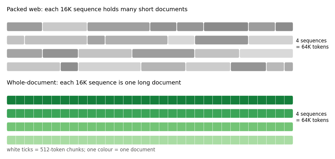
Both batches have the same number of tokens, so on paper they are the same batch size. But the 32 chunks of one repository are not 32 independent samples. They share variable names, style, topic and imports. If their gradients point the same way, averaging them cancels less noise than averaging 32 unrelated chunks would.
The idea in one formula
Survey statisticians have a name for this: the design effect. If you sample people in clusters (whole households, whole schools) instead of one by one, your estimate is noisier than the sample size suggests. For a block of m chunks whose noise is correlated, the variance of their average is
Here σ² is the noise of one chunk's gradient and ρ is the correlation between two chunks' noise. If the chunks were independent, R would be 1. If R = 4, your batch carries as much noise as one with a quarter of the samples. In the language of McCandlish et al., R is how much the noise scale Bsimple grows when you swap shuffled chunks for whole-document blocks of the same corpus.
How I measured it
The plan was frozen before any gradient was computed, and it is public. One rule was added later, after part of the data had been seen; that is explained under What went wrong. The setup:
| models | Pythia-410M (4 checkpoints), Pythia-1.4B (2), OLMo-2-1B (2) |
|---|---|
| corpora | code repositories (The Stack, concatenated by repo), arXiv papers, PG-19 books, and packed FineWeb as the control |
| sample | 16 documents per corpus, the same 16 for every model; from each, the span from token 2,048 to 18,432, cut into 32 chunks of 512 tokens |
| per cell | 512 chunk gradients and their inner products (a Gram matrix) |
| coverage | 32 planned cells: 24 complete, 5 partial, 3 missing; every final checkpoint is complete |
| hardware | CPU only, 4-core cloud machines; no GPU |
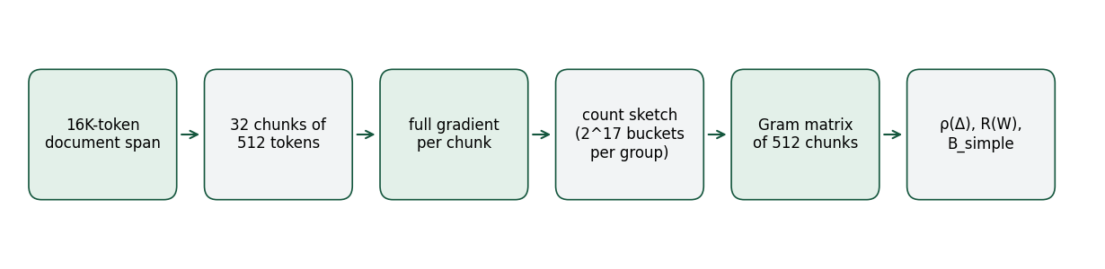
That last point cuts both ways. It keeps the measurement clean, but it also means this is not the gradient of a real 16K training sequence, where each chunk sees everything before it. The numbers here describe batches of 512-token chunks grouped by document. They are a proxy for long-context training, and the real multiplier could be larger or smaller.
A full gradient has hundreds of millions of numbers, and storing 512 of them per cell was not an option on CPUs. So each gradient is compressed with a count sketch: every parameter is hashed into one of 131,072 buckets with a random sign, separately for attention, MLP, embedding and other parameters. Inner products survive this almost exactly. Exact squared norms are kept on the side.
From the inner products, three things fall out. Pairs from different documents give the squared length of the mean gradient. The diagonal, minus that, gives the noise variance of one chunk. Pairs from the same document at distance Δ give the correlation ρ(Δ). For the two 1B models, documents were processed in groups of four, so only pairs inside a group exist: 24 of the 120 possible document pairs.
Result 1: the correlation reaches far
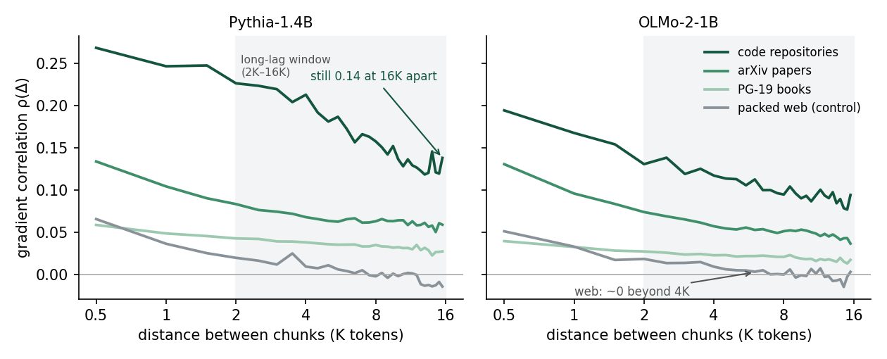
Two chunks of the same repository, about 16K tokens apart, still have a noise correlation of about 0.1: 0.14 on Pythia-1.4B and 0.09 on OLMo-2. ArXiv falls from 0.13 at 512 tokens to 0.07–0.08 at 2K and 0.04–0.06 at the longest distance. Books are lower but clearly positive. The web control behaves as you would expect from packing: some correlation at short range, where one web document spans neighbouring chunks, and essentially zero beyond about 4K.
A correlation of 0.1 sounds small. It is not, because the design effect adds it up over every pair, and a 16K block has 496 pairs of chunks. These are averages over pairs and documents; individual pairs vary a lot.
Result 2: the noise grows with block length
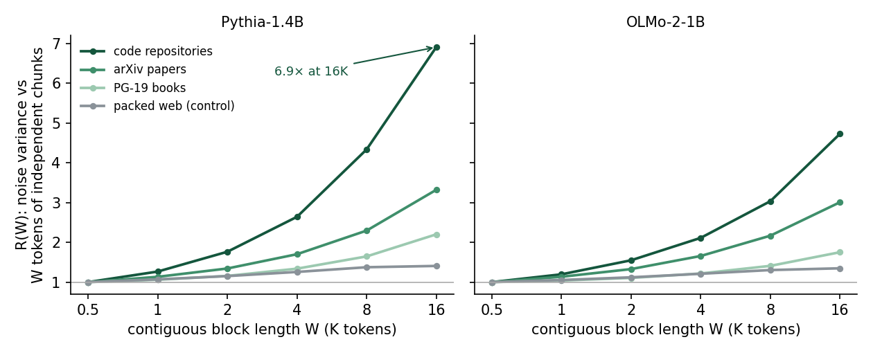
The longer the block, the more correlated pairs it contains, and the bigger the penalty. At 16K tokens a code block carries 4.7–6.9× the noise of independent chunks of the same code.
Result 3: against the control
The packed-web control is not at 1 either. Short web documents straddle chunk boundaries, which gives it R = 1.3–1.4. The fair comparison is therefore relative: each corpus divided by packed web at the same model and checkpoint, Rrel = Rcorpus / Rweb. Each R is measured against shuffled chunks of its own corpus, so Rrel compares how much each layout shrinks the sample count. It does not compare absolute noise levels between corpora; that would also need the ratio of their per-chunk noise variances, which is not part of this comparison.
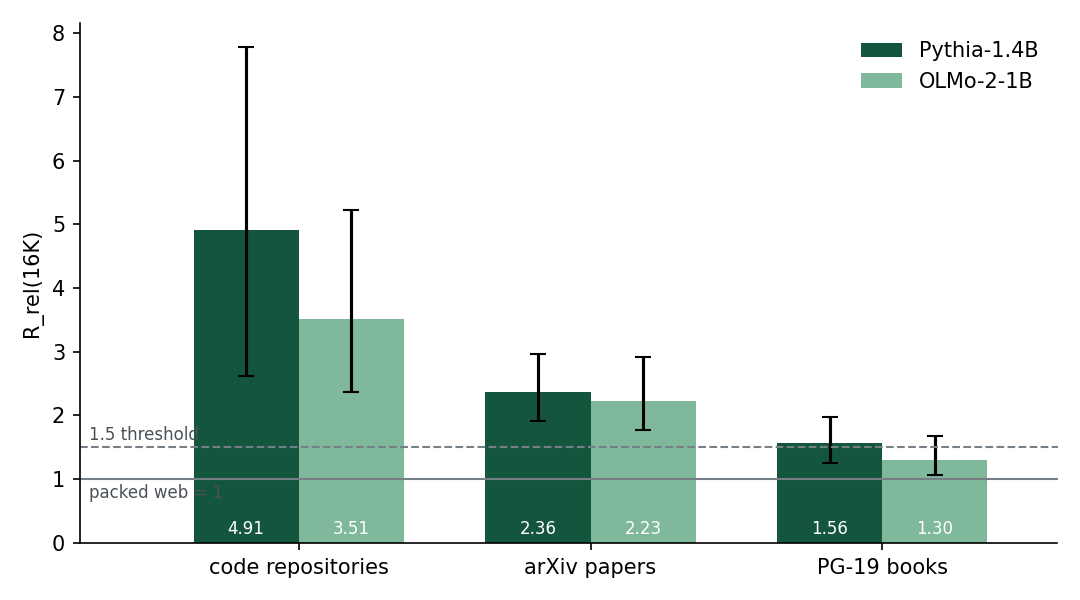
| corpus | Pythia-1.4B | OLMo-2-1B | raw R(16K) |
|---|---|---|---|
| code repositories | 4.91 [2.61, 7.78] | 3.51 [2.37, 5.23] | 6.91 / 4.73 |
| arXiv papers | 2.36 [1.91, 2.96] | 2.23 [1.78, 2.92] | 3.32 / 3.01 |
| PG-19 books | 1.56 [1.26, 1.98] | 1.30 [1.07, 1.67] | 2.20 / 1.75 |
| packed web | 1 | 1 | 1.41 / 1.35 |
The two models disagree on the exact size but agree on the order: code, then arXiv, then books. The intervals come from resampling the 16 documents with replacement, so they reflect only the documents I drew. Books sit near 1.5, the threshold the plan set in advance for raw R and the addendum later applied to Rrel.
The four corpora side by side
| loss (nats) | ρ at 512 tokens | ρ, 2K–16K average | R(16K) | per-document share: median / max | |
|---|---|---|---|---|---|
| Pythia-1.4B, final checkpoint | |||||
| code repositories | 1.14 | 0.27 | 0.16 | 6.91 | 0.07 / 1.06 |
| arXiv papers | 1.71 | 0.13 | 0.06 | 3.32 | 0.06 / 0.10 |
| PG-19 books | 2.76 | 0.06 | 0.03 | 2.20 | 0.03 / 0.07 |
| packed web | 2.93 | 0.07 | 0.00 | 1.41 | 0.00 / 0.05 |
| OLMo-2-1B, final checkpoint | |||||
| code repositories | 1.42 | 0.19 | 0.10 | 4.73 | 0.07 / 0.26 |
| arXiv papers | 1.78 | 0.13 | 0.05 | 3.01 | 0.05 / 0.09 |
| PG-19 books | 2.87 | 0.04 | 0.02 | 1.75 | 0.02 / 0.03 |
| packed web | 2.88 | 0.05 | 0.00 | 1.35 | −0.01 / 0.06 |
Note the web row: its short-range correlation (0.05–0.07 at 512 tokens) is as high as the books', but it vanishes at long range. The books are the reverse: weak, but it never goes away. The last column is each document's long-range term, scaled by the variance of the whole cell rather than its own, so it is not a correlation and can exceed 1.
What it means for your batch size
Turn the ratio around and you get an effective batch size: how many tokens of packed web would hold the same number of effective independent samples.
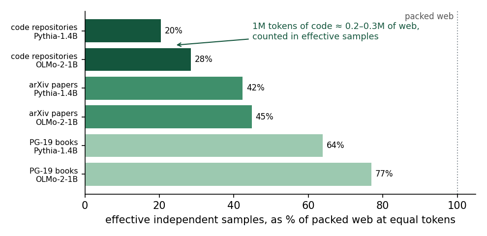
| 1M tokens per step of… | as many effective samples as (Pythia-1.4B) | (OLMo-2-1B) |
|---|---|---|
| whole code repositories | 204K web tokens [129K, 382K] | 285K web tokens [191K, 421K] |
| whole arXiv papers | 424K [337K, 523K] | 448K [342K, 562K] |
| whole books | 639K [504K, 793K] | 769K [597K, 932K] |
The brackets are the 95% intervals carried over from Rrel; the ranges in the text are the two models' point estimates. This matters because long-context data mixes lean heavily on code repositories. ProLong's long-document data, for instance, is mostly repositories and books. If you size a whole-document batch by its token count, as you would packed data, it may hold several times fewer independent samples than that count suggests.
Three cautions. These numbers count samples; they do not say that 1M tokens of code and 204K tokens of web have the same gradient noise in absolute terms, because a single code chunk and a single web chunk have different noise variance and different mean gradients. They come from 512-token chunks without long context, so they are a proxy for 16K training. And they do not give a learning-rate rule: Bsimple ignores curvature, and a noisier gradient does not by itself mean a worse model.
It is not only an early-training effect
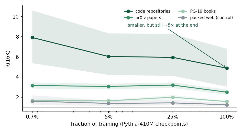
One worry was that this only shows up very early, when the model has not learned much and every gradient looks alike. On Pythia-410M it does not. The code effect shrinks over training, from about 8 to about 5, and arXiv falls by about a fifth, from 3.2 to 2.5, but the ordering holds at every checkpoint. For the two 1B models only the final checkpoints are complete, so this check rests on the smaller model.
It is lumpy
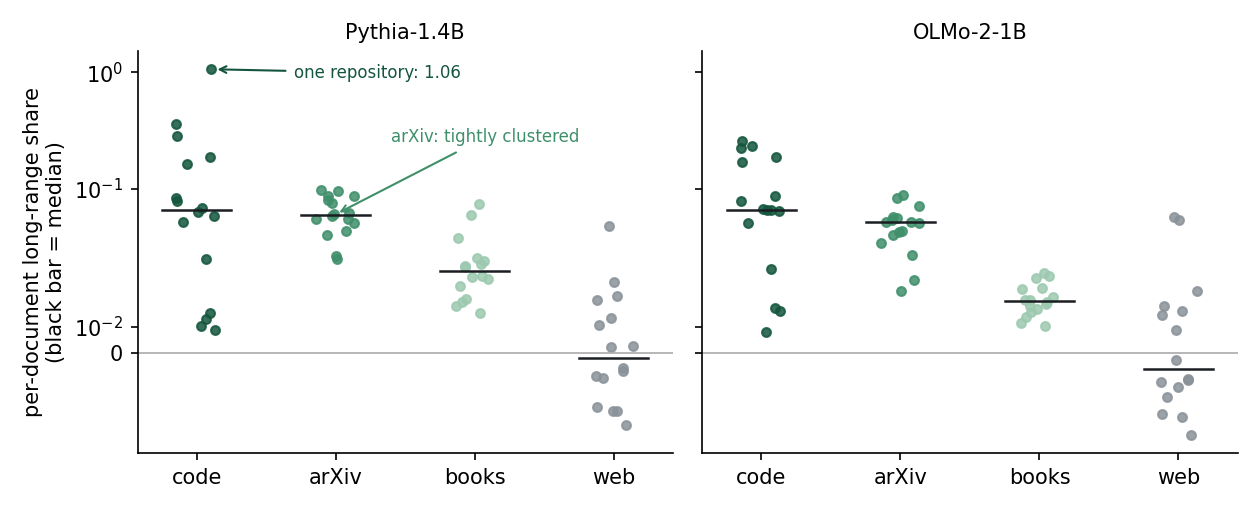
ArXiv papers are remarkably uniform: every one of the 16 sits near the median. Code repositories are not. A few repositories contribute a lot, and some barely anything. This is why the code intervals are so wide, and it suggests the effect depends a lot on which repositories you train on. A sixteen-repository sample is enough to see it, not enough to pin it down, and it says nothing about kinds of repositories it did not include.
It shows up in every parameter group
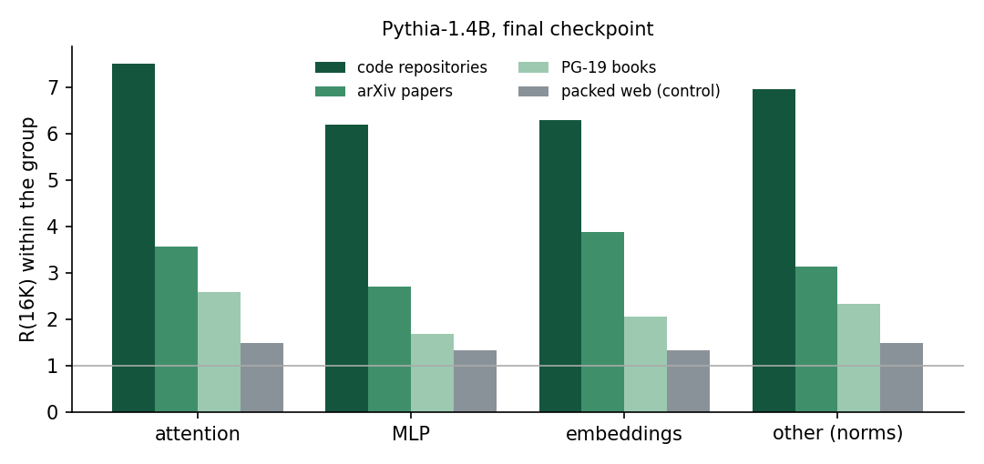
The penalty is not driven by one part of the model, say the embedding rows of rare tokens that keep recurring in one repository. Attention, MLP, embeddings and the remaining parameters all show it, in the same order. These are four large groups; I did not look at single layers or heads.
Checking the instrument
Two things could fake a result like this: a sketch that distorts inner products, or a position effect where chunks late in a sequence look different. The checks below argue against both, but they are narrower than a full validation.
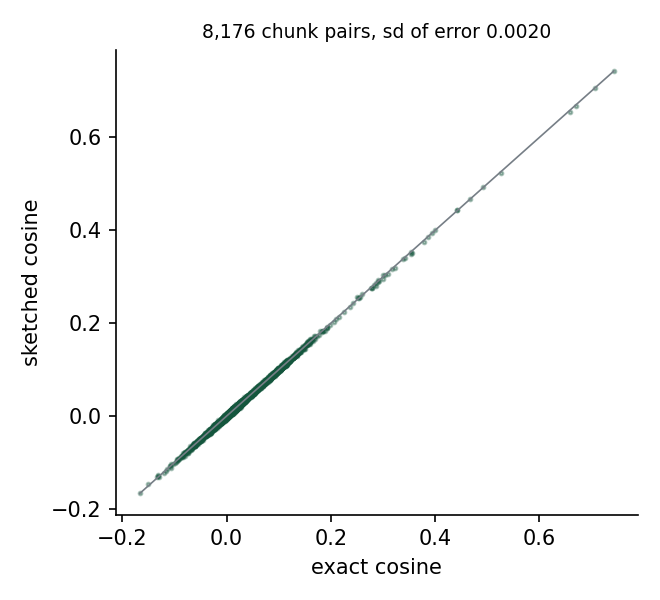
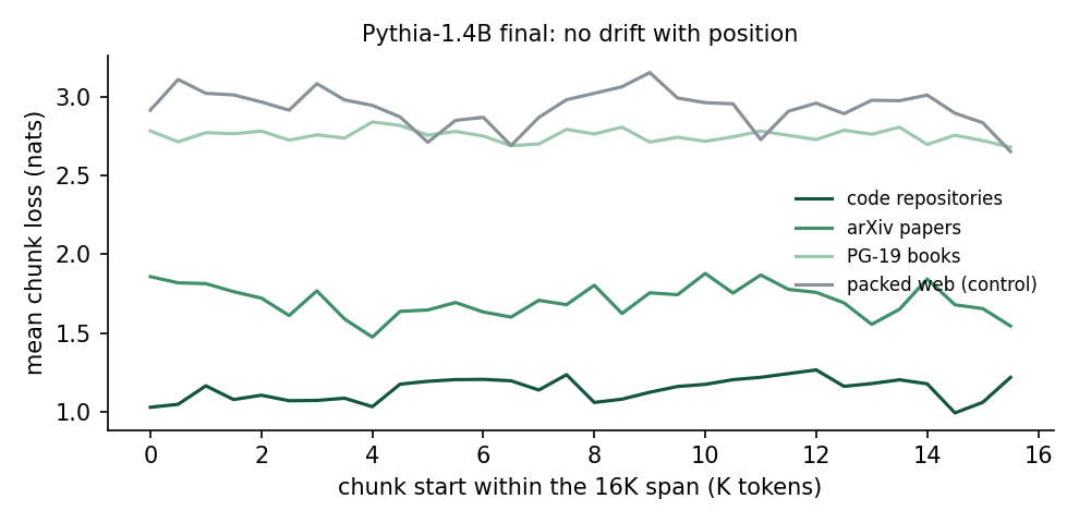
The sketch check was run on the smallest model only. Losses are flat across the span, which rules out the crudest position effect, though not every way a gradient could depend on position. They also show the familiar ordering: code is the easiest text for these models, at about 1.1 nats per token, and web the hardest, at about 2.9. Two more gates are worth naming. The web control's long-range correlation passes the plan's 0.01 limit on its point estimate, but its intervals reach 0.010–0.012. And one gate fails: for Pythia-1.4B books, the squared mean gradient is too uncertain (its interval includes zero), which makes Bsimple unreliable there. R does not divide by it.
An interactive version of this post, with a batch-size calculator and every curve, is at severinvisionary.github.io/doc-batch-gradients.
Try it yourself
Pick a corpus, a model and the tokens per step you train with. Then flip through the curves behind the numbers above.
What went wrong, and what I changed
Not everything went to plan, and the details are in the repository.
- The first sketch failed its own test. The preregistered sketch was a small Kronecker projection, and it failed the fidelity check during the trial run. I replaced it with the count sketch above, and wrote that down, before any real measurement.
- The control was not as clean as planned. The plan required packed web to come in below 1.2. At the final checkpoints it came in at 1.26–1.41, because of the short-range overlap described above. Under the original rules that makes the verdict inconclusive, and it stays so. I then added a control-relative rule, the Rrel above, in a written addendum. By then I had seen all of the Pythia-410M results and part of the 1B data, including half of the Pythia-1.4B web control (R(16K) = 1.59 on 8 documents), so the new rule is not fully blind. Under it, none of the plan's stopping criteria fire. That means the effect is large enough to be worth testing in training, not that it has been shown to matter there.
- Some early checkpoints are incomplete. Compute ran out for a few early 1B-scale cells: 5 are partial and 3 are missing. The final checkpoints, which carry the conclusion, are complete.
- One estimate is noisier than planned. For the 1B models, documents were processed in groups of four, so the mean gradient is estimated from pairs within those groups only.
What this does not show
Long-context training can cost some short-context quality, depending on the data mix; ProLong, for one, reports both the losses and mixes that avoid them. A noisier gradient is one possible reason. Others include attention spreading too thin over long windows, a mismatch between training and test lengths, and a plain shift in domain. This measurement shows the extra noise is there for 512-token chunks grouped by document, and how big it is. It does not measure the noise of real 16K-context gradients, and it does not show how much of any quality cost the noise explains.
Testing that takes training runs. One design changes only how a fixed set of documents is cut and batched:
| arm | window | documents per step | what it changes |
|---|---|---|---|
| A | 16K, whole documents | 64 | the usual long-context setup |
| B | 1K, the same 64 documents chopped, accumulated into one update | 64 | A vs B: the window, with batch content fixed |
| C | 1K, chunks shuffled across the same pool of documents | ~1,000 | B vs C: batch composition, with the window and the token pool fixed |
All three arms need the same tokens, the same number of updates and the same exposure to each document over training. If each explanation acted alone, you would expect roughly this:
| explanation, acting alone | A vs B (window) | B vs C (composition) |
|---|---|---|
| design effect (this post) | about equal | C better |
| the long window itself hurts | A worse | about equal |
| train/test length mismatch | A worse on short evals only | about equal |
In practice these can act together, and A and B differ in more than noise, since longer context changes the gradient itself. A gap between B and C would show that batch composition matters, not by itself that this design effect is the reason. This would take a few thousand GPU-hours at the 400M–1B scale. I have not run it.
Related work
- Everett and Qiu (arXiv 2609.04577, Appendix I) point out that tokens in one sequence share context and are likely more correlated. They suggest comparing batch-size and length splits at matched tokens.
- McCandlish et al. (arXiv 1812.06162) define the noise scale Bsimple used here.
- Thomas (arXiv 2607.05872) uses a shuffled-document control on real language-model gradients and finds that within-document correlation explains only a small part of the gradient-spectrum effect studied there. It does not measure correlation by distance or a design effect.
- Work on critical batch size (arXiv 2410.21676) finds little sensitivity to context length, on packed data and contexts up to 4K.
- Dataset Decomposition (arXiv 2405.13226) and ProLong (arXiv 2410.02660) study length curricula and long-document data mixes. They do not measure gradient correlation.
I could not find an earlier measurement of within-document gradient correlation as a function of distance, or of the design effect it implies, on real language-model gradients. If you know of one, I would like to hear about it.
Data and code
Everything is in doc-batch-gradients: the probe,
the analysis, the Gram matrices for all 57 shards, and the full report. Every number on this page can be
recomputed on a laptop in about 20 minutes. The plan, the deviations and the addendum are in docs/.
How to cite
This post, the code and the analysis report are archived on Zenodo as doi:10.5281/zenodo.23270769. The Gram matrices are too large for that deposit; they stay in the GitHub repository at tag v2.0, and the deposit lists their SHA-256 hashes.
@techreport{yang2026longdocbatch,
  author = {Yang, Hanyu},
  title  = {Long documents make your batch smaller than it looks: measuring within-document gradient correlation},
  year   = {2026},
  institution = {Zenodo},
  doi    = {10.5281/zenodo.23270769},
  url    = {https://doi.org/10.5281/zenodo.23270769}
}